Advanced analysis of kinetic reactions

6.5 Advanced analysis of kinetic reactions

This last section of the lecture is full of math. Some will enjoy it. Others will practice the techniques for solving sets of linear differential equations with constant coefficients and typical approximation to simplify the solutions for limiting cases, thus allowing for a deeper understanding of kinetics. You will need it in the future!
For the complete reaction scheme in Eq. (6.10) leading to the set of first order differential equations

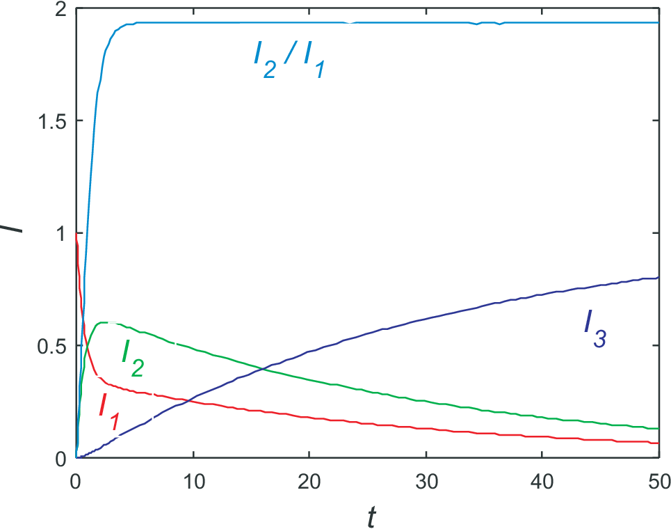
\begin{equation*} \frac{dI_1}{dt} = - k_1 I_1 + k_3 I_2 \quad , \quad \frac{dI_2}{dt} = k_1 I_1 - k_3 I_2 - k_2 I_2\quad \mbox{, and} \quad \frac{dI_3}{dt} = + k_2 I_2 \label{kin_3a} \end{equation*}

(6.22)

an example for the solution is shown in Fig. (6.2). As starting values we choose \(I_1(0)=1\), \(I_2(0)=0\), and \(I_3(0)=0\). The values for the kinetic coefficients are \(k_1=1\), \(k_3=0.5\), and \(k_2=0.05\).
In what follows we will discuss in more details the three concepts often used to describe transport and kinetics:

rate limiting step
pre- steady state condition
steady state

Figure 6.2: Numerical solution of the set of differential equations: \(I_1(t)\), \(I_2(t)\), \(I_3(t)\), and the ratio \(I_2(t)/I_1(t)\).

The rate limiting step is always the slowest process, i.e. that with the smallest kinetic coefficient, in our case \(k_2\). Somehow counter intuitively not the large kinetic coefficients dominate the time dependencies, but the slowest process needs the longest time to reach steady state.
Steady state means that no changes in time exist, i.e. all derivatives on the left hand side of the set of differential equations are zero. From the third equation we find \(I_2(t\to\infty)=0\). Therefore from the first equation we find \(I_1(t\to\infty)=0\). From particle conservation we find \(I_3(t\to\infty)=1\). This are the relations visualized in Fig. 6.2; additionally the ration of \(I_2/I_1\) is shown. Obviously this ratio reaches a constant value long before steady state is reached. This effect is called pre-steady state condition and is implied by the large kinetic coefficients \(k_1\) and \(k_3\). Taking for the moment \(k_2=0\) the (pre-) steady state condition is reached for \(dI_1/dt = dI_2/dt=0\), i.e. \(k_1/I_1 = k_3/I_2\) or \(I_2/I_1 = k_1/k_3\). This value is close to the ration visible in Fig. 6.2. It corresponds to the result already discussed before in Eq. (6.15). Actually we have discussed the result in zeros order on \(k_2\), ignoring completely the time dependence \(dI_1/dt\) and \(dI_2/dt\). We can significantly improve the approximation by an analysis in linear order in \(k_2\). Let us write

\begin{equation*} I_2 = \frac{k_1-\Delta}{k_3}I_1 \quad \mbox{i.e.} \quad \frac{dI_2}{dt}= \frac{k_1-\Delta}{k_3} \frac{dI_1}{dt} - \frac{1}{k_3} \frac{d\Delta}{dt} I_2 \approx \frac{k_1-\Delta}{k_3} \frac{dI_1}{dt} \end{equation*}

(6.23)

The last equation holds for pre-steady state since in this regime the ration between \(I_2\) and \(I_1\) is constant, i.e. \(\Delta\) is constant. Including this into the set of differential equations we get

\begin{equation*} \begin{split} \frac{dI_1}{dt} & = - \Delta\; I_1\\ \frac{dI_2}{dt} & = + \Delta\; I_1 - k_2\;\frac{k_1-\Delta}{k_3}I_1\\ \frac{dI_3}{dt} & = + \;k_2\;\frac{k_1-\Delta}{k_3}I_1\\ \end{split} \label{eq:reaction_scheme} \end{equation*}

(6.24)

So for pre-steady state we find

\begin{equation*} \frac{k_1-\Delta}{k_3} = \frac{I_2}{I_1} \approx \frac{dI_2/dt}{dI_1/dt} = - \frac{\Delta-k_2\frac{k_1-\Delta}{k_3}}{\Delta} \end{equation*}

(6.25)

i.e.

\begin{equation*} k_1\;\Delta-\Delta^2 = -k_3\;\Delta + k_2 (k_1-\Delta) \end{equation*}

(6.26)

Since we discuss the problem in linear order in \(k_2\), i.e. \(\Delta \propto k_2\), we ignore \(\Delta^2\) (it is tiny!) and find

\begin{equation*} \Delta = k_2\;\frac{k_1}{k_1+k_3+k_2} \end{equation*}

(6.27)

So at pre-steady state

\begin{equation*} I_2 = \frac{k_1}{k_3}\;\frac{k_1+k_3}{k_1+k_3+k_2}\;I_1 \quad , \end{equation*}

(6.28)

somewhat smaller than for \(k_2=0\).
For the set of differential equations we find

\begin{equation*} \begin{split} \frac{dI_1}{dt} & = - k_2\;\frac{k_1}{k_1+k_3+k_2}\; I_1 \quad \Rightarrow \quad I_1(t) = I_0 \exp \left(-\frac{k_2\,k_1}{k_1+k_3+k_2} t\right)\\ \frac{dI_2}{dt} & = - k_2\;\frac{k_1}{k_3}\;\frac{k_1}{k_1+k_3+k_2}\;I_1 \quad \mbox{i.e.} \quad I_2(t) = \frac{k_1}{k_3}\;\frac{k_1+k_3}{k_1+k_3+k_2}\;I_1(t)\\ \frac{dI_3}{dt} & = + k_2\;\frac{k_1}{k_3}\;\frac{k_1+k_3}{k_1+k_3+k_2}\;I_1 \quad \mbox{i.e.} \quad I_3(t) = I_0 \left[1 - \left(1+\frac{k_1+k_3}{k_1+k_3+k_2} \right) \exp \left(-\frac{k_2\,k_1}{k_1+k_3+k_2} t \right) \right]\\ \end{split} \label{lin_version_chem_ode} \end{equation*}

(6.29)

which in a very good approximation reflect the numerical solutions in Fig. 6.2. So as typical we can use the exact numerical results to identify possible simplifications to find good/reasonable analytic approximation of the numerical results. Here we learned most from the constant ratio of \(I_2/I_1\) for nearly the whole time of the reaction.
Finally we will calculate the full solution of the Eqs. (6.24) without the back reaction, i.e. \(k_3=0\). For \(I_1\) we get

\begin{equation*} I_1(t) = I_0 \exp(-k_1\,t) \quad. \end{equation*}

(6.30)

Including this into the second ode we get

\begin{equation*} \frac{d I_2}{dt} = k_1 I_0 \exp(-k_1\,t) - k_2 I_2 \quad. \end{equation*}

(6.31)

The solution of the homogeneous ode is of course

\begin{equation*} I_2(t) = D \exp(-k_2\,t) \quad. \end{equation*}

(6.32)

To find a particular solution of the inhomogeneous ode routinely a variation of the constant is used, i.e. an approach

\begin{equation*} I_2(t) = D(t) \exp(-k_2\,t) \quad \mbox{i.e.} \quad \frac{d I_2}{dt} = \frac{d D}{dt} \exp(-k_2\,t) - D(t) k_2 \exp(-k_2\,t) \quad. \end{equation*}

(6.33)

Including this into the ode we find

\begin{equation*} \frac{d D}{dt} = k_1 I_0 \exp\left((k_2-k_1)\,t \right) \quad. \end{equation*}

(6.34)

i.e.

\begin{equation*} D(t) = \frac{k_1 I_0}{k_2-k_1} \exp\left((k_2-k_1)\,t \right) + const. \quad, \end{equation*}

(6.35)

leading to

\begin{equation*} I_2(t) = \left[\frac{k_1 I_0}{k_2-k_1} \exp\left((k_2-k_1)\,t \right) + const.\right] \exp(-k_2\,t) \quad, \end{equation*}

(6.36)

Taking into account the starting condition \(I_2(0)=0\), we get

\begin{equation*} const. = -\frac{k_1 I_0}{k_2-k_1} \quad , \end{equation*}

(6.37)

and find

\begin{equation*} I_2(t) = \frac{k_1 I_0}{k_2-k_1} \left[ \exp\left(-k_1\,t \right) - \exp\left(-k_2\,t \right)\right] \quad. \end{equation*}

(6.38)

Finally from particle conservation \(I_0 = I_1(t) + I_2(t) + I_3(t)\) we get

\begin{equation*} I_3(t) = I_0 \left[ 1 - \frac{k_2\,\exp\left(-k_1\,t \right) + k_1\,\exp\left(-k_2\,t \right)}{k_2-k_1}\right] \quad. \label{eq:I_3sol} \end{equation*}

(6.39)

Since the principle behavior significantly changes for different combination of \(k_1\) and \(k_2\) we will discuss three limiting cases:

For \(k_1 \to k_2\) we can rewrite

\begin{equation*} \begin{split} I_2(t) &= \frac{k_1\, I_0}{k_2-k_1} \exp\left(-k_1\,t \right) \left[ 1 - \exp\left(-(k_2-k_1) t \right) \right] \\ & \approx k_1\, I_0 \exp\left(-k_1\,t \right) \frac{1-\left(1-(k_2-k_1) t \right)}{k_2-k_1} = k_1\, I_0 \exp\left(-k_1 t \right) t \quad. \end{split} \end{equation*}

(6.40)

Here we developed the exponential function up to linear order in \((k_2-k_1)\) and find astonishingly a linear component in the solution. Including this result into Eq. (6.39) we find

\begin{equation*} I_3(t) = I_0 \left[ 1 - \exp\left(-k_1\,t \right)(1+t) \right] \quad. \end{equation*}

(6.41)

For \(k_1 \gg k_2\) we find easily

\begin{equation*} I_2(t) = I_0 \exp\left(-k_2\,t \right) \quad \mbox{and} \quad I_3(t) = I_0 \left[1-\exp\left(-k_2\,t \right)\right] \quad. \end{equation*} (6.42)

For \(k_1 \ll k_2\) we find easily

\begin{equation*} I_2(t) = \frac{k_1}{k_2} I_0 \exp\left(-k_1\,t \right) = \frac{k_1}{k_2} I_1(t) \quad \mbox{and} \quad I_3(t) = I_0 \left[1-\exp\left(-k_1\,t \right)\right] = I_0 - I_1(t) \quad. \end{equation*}

(6.43)

Here we again see nicely the effect of the rate limiting process described by a small value of \(k_1\) and the pre-steady state condition \(I_2(t)/I_1(t)=k_1/k_2\).