Solution to Exercise 4.2-1 "Diffusion During Cooling"

	For the diffusion length L we have the well known equations:
		E is the activation energy of the diffusing species an k is the Boltzmann constant. Because of T = T0 · exp –(l · t) we obtain for L2
	Now we have a purely mathematical exercise which is not too difficult, but not too easy either. In order to solve the integral, we try the substitution
		The boundaries must be changed too, we obtain t = 0 changes to u0 = E/kT0 t = ¥ changes to u = ¥. This gives us

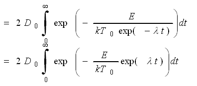
	Now you must solve a simple looking integral. There are several ways of doing that
		Find a good math book with lots of integrals and take the solution from there (the "Bronstein", however, won't do) Do a sensible approximation and solve it yourself in a simple way Go all the way and solve it completely - if you can.
		Here we go the second route.
	We use a Taylor expansion for 1/u around u0 because that's where u is felt most critically - for large values of u everything tends to be zero anyway. In full generality we have
		If we keep it really simple, we could just use the first term, having 1/u » 1/u0; but we will go one step beyond this and take
		1 u   »  1 u0  –    u  –  u0 u02
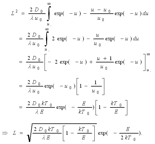
		This gives us
		The second term of the Taylor expansion brought in the factor [1 – kT0/E] and since kT0 « E in all normal cases, it is indeed not very important. If we neglect it, we may simply give the desired solution as
		L = æ ç è 2D0 · kT0 l · E ö ÷ ø 1/2  ·  exp       E  2kT0

	Now we can look at some typical cases and see what this formula means. However, first we have to find the right values for l
		For this we have to take the given values of the initial cooling rate, which we call l', and see what l values correspond to these cooling rates.
		The initial cooling rate l' is the derivative of the T(t) function at t = t0 = 0, we thus have
		d dt (T0 · exp – l · t ÷ ÷ t  =  0  =   l'  =   – l ·T0 · exp –l · t ÷ ÷ t = 0  =  – l ·T0
		and obtain
		l  =  l' T0
		The "–" sign cancels, because our l' must carry a minus sign, too, if it is to be a cooling and not a heating rate.
	Replacing l by l'/T0 yields the final formula:
		L  =   æ ç è 2D0 · kT02 l' · E ö ÷ ø 1/2  ·  exp       E  2kT0
		We have to evaluate this formula for cooling rates l' given as (–) 1 oK/s, 10 oK/s, 50 oK/s, 104 oK/s, and activation energies of E = 1.0 eV, 2.0 eV, 5 eV. For D0 we take D0 = 10–5 cm2s–1.
		The result (including the [1 – kT0/E] term is shown below
	What can we learn from the formula and the curves?
		The cooling rate is not all that important. Differences in the cooling rate of a factor of 50 produce only an order of magnitude effect or less since L is only proportional to (1/l)1/2. The starting temperature T0 is slightly more important than the activation energy E; both have the same weight in the exponential, but T0 appears directly in the pre-exponential while E enters only as square root. The pre-exponential factor D0 of the diffusion coefficient is exactly as important as l' and E in the pre-exponential factor of the equation for L
		What can we do with the numbers? Quite simple: L gives you the average of the largest distance between some point defect agglomerates, e.g. precipitates, because point defects farther away than L from some nuclei cannot reach it and must form their own agglomerate. The average number of point defects in an agglomerate divided by L3 gives a lower limit for the point defect concentration, because at least as many point defects as we find in an agglomerate must have been in the volume L3.

With frame

Exercise 4.2-1 Diffusion During Cooling

Exercise 4.1-1 Lifetime of Positrons

© H. Föll (Defects - Script)