This method is an algorithm to find a zero of a function by repeated bisection of an interval and determination of the sub interval where the zero must be found. It is simple and reliable, but relatively slow.
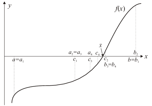
Consider an interval \([a,b]\) and a function \(f\) that has different signs at the boundaries of that interval: \(f(a)\,f(b)\lt0\) (cf. Fig. 3.1). Therefore, for a continuous function \(f\) there must be at least one zero within the interval \([a,b]\). To numerically approach a zero \(\bar{x}\) of \(f\), the midpoint of the interval is taken as first approximation (with \(a_1 = a\), \(b_1 = b\)):
|
| \begin{equation*} c_1= a_1+\frac{b_1-a_1}{2}=\frac{b_1+a_1}{2}\,. \end{equation*} | (3.7) |
The maximum absolute error of this approximation obviously is half of the original interval width:
|
| \begin{equation*} \left|c_1-\bar{x}\right|\leq \frac{b_1-a_1}{2}\,. \end{equation*} | (3.8) |
If this error is considered too large, one has to repeat the bisection for the subinterval where the zero must be found. It can be determined from a change of sign of \(f\), which can occur for one of the sub intervals only (either for \([a_1,c_1]\) or for \([c_1,b_1]\)). This determines the choice of the interval \([a_2,b_2]\) for the next step:
|
| \begin{equation*} \begin{split} f(a_1)\,f(c_1)\lt 0 & \Rightarrow a_2 = a_1,\ b_2 = c_1;\\ f(c_1)\,f(b_1)\lt 0 & \Rightarrow a_2 = c_1,\ b_2 = b_1. \end{split} \end{equation*} | (3.9) |
|
| \begin{equation*} \left|c_2-\bar{x}\right|\leq \frac{b_2-a_2}{2} = \frac{b_1-a_1}{4}\,. \end{equation*} | (3.10) |
If accidentally at some step \(k\) the midpoint is the sought-after zero, then \(f(a_k)\,f(c_k) = f(c_k)\,f(b_k) = 0\) and the iteration must stop. However, see also remark 3 below.
If \(a_n, b_n, c_n\) are the relevant values for the \(n^{\text{th}}\) step, then (remember that \(a_1 = a\), \(b_1 = b\))
|
| \begin{equation*} b_n-a_n = \frac{b-a}{2^{n-1}}\,, \quad \left|c_n-\bar{x}\right|\leq \frac{b_n-a_n}{2} = \frac{b-a}{2^n}\,. \end{equation*} | (3.11) |
Since \(\lim_{n \to \infty} \frac{1}{2^n}=0\), one has that \(\lim_{n \to \infty}\{c_n\} = \bar{x}\), i.e. this method converges. Since in each step the maximum absolute error is reduced by a factor \(\frac{1}{2}\), the convergence behavior is called linear with a factor \(\frac{1}{2}\). This factor is also called rate of convergence.
The advantage of the bisection method is that it always converges. However, it is a slow process. To reach a maximum error \(\left|c_n-\bar{x}\right|\leq \epsilon\) with a given \(\epsilon\) corresponds to \((b-a)/2^n\leq\epsilon\). Therefore, one can determine the number of necessary bisection steps from \(2^n \geq (b-a)/\epsilon\) as
|
| \begin{equation*} n \geq \log_2\frac{b-a}{\epsilon}\,. \end{equation*} | (3.12) |
Remark 1:
non-detectable zeros
The interval bisection method relies on a
change of the sign of \(f\). However, \(f\) might have a zero where the sign does not change,
i.e. where the graph does not cross the \(x\) axis but an osculation occurs (as, e.g., at the extremum
of a parabola). Such a second-order
zero cannot be found by the interval bisection method.
Remark 2:
multiple zeros
The interval bisection method always converges to
a zero of \(f\). However, \(f\) might have several zeros in \([a,b]\). This will
not be noticed by the interval bisection method, which therefore will find only one of them—but it is not clear which
one will be found.
Remark 3:
numerical stability
To detect a change of the sign of \(f\),
the interval bisection algorithm is formulated above in terms of a product of two function values. Since a zero of \(f\) is approached, these values can become very small, so that their product may lead to numerical underflow. This
can furthermore be confused with the case that accidentally the midpoint is the sought-after zero, i.e. not the product
but already a single function value equals zero. A robust numerical implementation must take care of these possibilities
and should not use products of function values.
Remark 4:
numerical accuracy
In general, the best accuracy that can be reached
for the value of the zero does not
equal the machine precision. This is related to the influence of the limited precision of floating-point arithmetic:
The larger a number (by absolute amount), the larger its exponent
will be, which means that the last digit of its mantissa will represent a larger value than for smaller numbers.
Therefore, because of always having the same (or a similar) number of significant digits available independent of the absolute
value, the absolute error of large numbers must in general be larger than that of small numbers. Because of that, only the
relative
error can be used as a measure of numerical accuracy (i.e. to determine when to end the iteration; an example
will be given in Sect. 5.1 below). In other words, the machine precision determines the smallest relative error reachable.
Specifying an \(\epsilon\) for the relative error smaller than the machine precision does not make sense and
should be prevented. But see also remark 5 below.
Remark 5:
numerical reliability
Additionally, not only the deviation with
respect to the \(x\) value might be of interest: It may happen that the function has a rather steep slope at
the zero, so that despite of a small relative error, \(\left|c_n-\bar{x}\right|/|\bar{x}|\leq \epsilon \ll
1\), a function value \(f(c_n)\) may occur that is still large. Therefore it is advisable to check this after
a zero has been determined numerically.
On the other hand, if the function has a rather
low slope at the zero, the interval of very small function values can be rather large, which implies that the problem of
numerical underflow described in remark 3 above might occur already before the prescribed accuracy has been reached. Then,
the algorithm will most likely exit with an unreliable value. Obviously, in such a case it does not make sense to specify
too small an \(\epsilon\) for the relative error.
General remark:
common problems
The problems treated in remarks 1 through 5 above
(roughly: existence and well-definedness of a solution for a certain algorithm, numerical stability/accuracy/reliability
of the respective implementation) are not only related to the subject of finding zeros, but apply to numerical problems
in general.
© J. Carstensen (Comp. Math.)