Exercise 7

9.7 Exercise 7

A theoretical introduction to solving numerically ODE is given in section 7.1. Here we will discuss examples of ODE of second order. Our first example is

\begin{equation*} \label{ode_sin_cos} \frac{d^2 y}{dt^2} = -y \end{equation*}

(9.12)

Translate the above differential equation of second order into a set of differential equations of first order
Check MATLAB HELP for ode45. Here you will find an example very close to the above problem
Copy the corresponding lines into a function and adapt the starting values to find cos(\(x\)) as the solution to the above problem
Adapt the starting values to find sin(\(x\)) as the solution to the above problem
Change the program to find exp(\(x\)) as solution
Change the program to find exp(\(-x\)) as solution
Change the program to find sinh(\(x\)) as solution
Change the program to find cosh(\(x\)) as solution

 function [T,Y] = mydglsolv

    [T,Y] = ode45(@myodefun,[0 2.*pi],[1 0]);
    plot(T,Y(:,1),’-’,T,Y(:,2),’-.’);
  
    function dy = myodefun(t,y)
       dy = zeros(2,1);
       dy(1)=y(2);
       dy(2)=-y(1);
    end
  
 end

Our next example is a reaction scheme specifying three kinetic coefficients \(k_1\), \(k_2\), and \(k_3\) for the following reaction chain

\begin{equation*} {\rm I}_1 \underset{k'}{\overset{k_1}{\rightleftharpoons}} {\rm I}_2 \xrightarrow{k_3} {\rm I}_3 \quad . \label{reaction_scheme} \end{equation*}

(9.13)

Assuming all reactions to be of first order this scheme translates into a set of differential equations

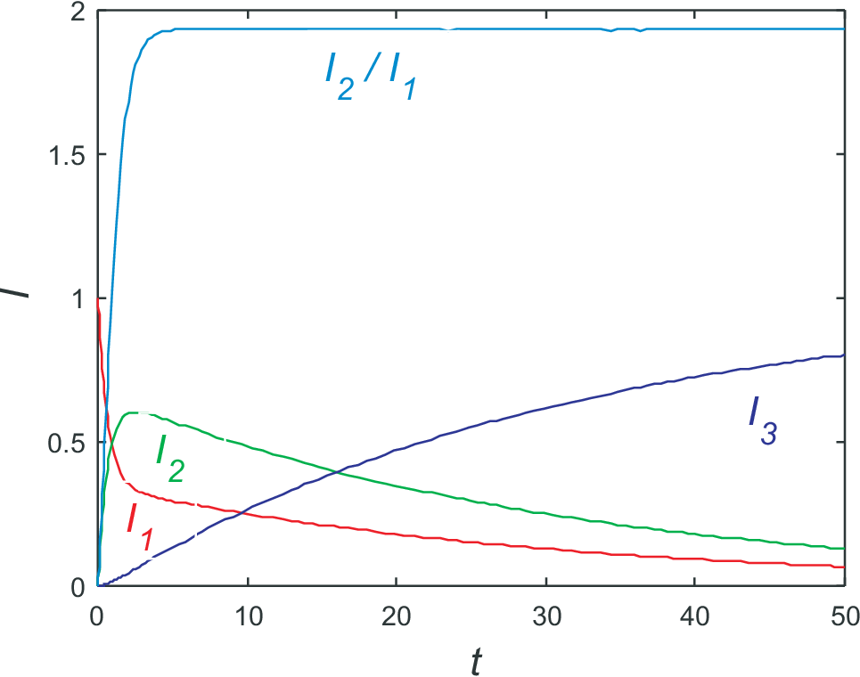
\begin{equation*} \frac{dI_1}{dt} = - \;k_1\,I_1 + \;k_2\;I_2 \quad , \quad\frac{dI_2}{dt} = + \;k_1\,I_1 - \;k_2\;I_2 -\;k_3\;I_2 \quad , \quad\frac{dI_3}{dt} = + \;k_3\;I_2 \quad . \end{equation*}

(9.14)

As starting values we choose \(I_1(0)=1\), \(I_2(0)=0\), and \(I_3(0)=0\). As kinetic coefficients we take \(k_1=1\), \(k_2=0.5\), and \(k_3=0.05\). The implementation in MATLAB is easy:

 function [T,Y] = my_chemical_odesolv
    k1=1;
    k2=0.5;
    k3=0.05;
    [T,Y] = ode45(@myodefun,[0 100],[1 0 0]);
    plot(T,Y(:,1),’-’,T,Y(:,2),’-.’);
  
    function dy = myodefun(t,y)
       dy = zeros(3,1);
       dy(1)=-k1.*y(1)+k2.*y(2);
       dy(2)=+k1.*y(1)-k2.*y(2)-k3.*y(2);
       dy(3)=+k3.*y(2);
    end
  
 end

Figure 9.3: Numerical solution of the set of differential equations: \(I_1(t)\), \(I_2(t)\), \(I_3(t)\), and the ratio \(I_2(t)/I_1(t)\).

The solution are shown in Fig. 9.3. In what follows we will briefly discuss three concepts often used for discussing transport and kinetics:

rate limiting step
pre- steady state condition
steady state

The rate limiting step is always the slowest process, i.e. that with the smallest kinetic coefficient, in our case \(k_3\). Somehow counter intuitively not the large kinetic coefficients dominate the time dependencies, but the slowest process needs the longest time to reach steady state.
Steady state means that no changes in time exist, i.e. all derivatives on the left hand side of the set of differential equations are zero. From the third equation we find \(I_3(t\to\infty)=0\). Therefore from the first equation we find \(I_1(t\to\infty)=0\). From particle conservation we find \(I_3(t\to\infty)=1\). This are the relations visualized in Fig. 9.3; additionally the ration of \(I_2/I_1\) is shown. Obviously this ratio reaches a constant value long before steady state is reached. This effect is called pre-steady state condition and is implied by the large kinetic coefficients \(k_1\) and \(k_2\). Taking for the moment \(k_3=0\) the (pre-) steady state condition is reached for \(dI_1/dt = dI_2/dt=0\), i.e. \(k_1/I_1 = k_2/I_2\) or \(I_2/I_1 = k_1/k_2\). This value is very close to the ration found from Fig. 9.3. The deviation can easily be understood from an analysis in linear order in \(k_3\). We will write

\begin{equation*} I_2 = \frac{k_1-\Delta}{k_2}I_1 \quad \mbox{i.e.} \quad \frac{dI_2}{dt}= \frac{k_1-\Delta}{k_2} \frac{dI_1}{dt} - \frac{1}{k_2} \frac{d\Delta}{dt} I_2 \approx \frac{k_1-\Delta}{k_2} \frac{dI_1}{dt} \end{equation*}

(9.15)

The last equation holds for pre-steady state since in this regime the ration between \(I_2\) and \(I_1\) is constant, i.e. \(\Delta\) is constant.
Including this into the set of differential equations we get

\begin{equation*} \begin{split} \frac{dI_1}{dt} & = - \Delta\; I_1\\ \frac{dI_2}{dt} & = + \Delta\; I_1 - k_3\;\frac{k_1-\Delta}{k_2}I_1\\ \frac{dI_3}{dt} & = + \;k_3\;\frac{k_1-\Delta}{k_2}I_1\\ \end{split} \end{equation*}

(9.16)

So for pre-steady state we find

\begin{equation*} \frac{k_1-\Delta}{k_2} = \frac{I_2}{I_1} \approx \frac{dI_2/dt}{dI_1/dt} = - \frac{\Delta-k_3\frac{k_1-\Delta}{k_2}}{\Delta} \end{equation*}

(9.17)

i.e.

\begin{equation*} k_1\;\Delta-\Delta^2 = -k_2\;\Delta + k_3 (k_1-\Delta) \end{equation*}

(9.18)

Since we discuss the problem in linear order in \(k_3\), i.e. \(\Delta \propto k_3\), we ignore \(\Delta^2\) (it is tiny!) and find

\begin{equation*} \Delta = k_3\;\frac{k_1}{k_1+k_2+k_3} \end{equation*}

(9.19)

So at pre-steady state

\begin{equation*} I_2 = \frac{k_1}{k_2}\;\frac{k_1+k_2}{k_1+k_2+k_3}\;I_1 \quad , \end{equation*}

(9.20)

somewhat smaller than for \(k_3=0\).
For the set of differential equations we find

\begin{equation*} \begin{split} \frac{dI_1}{dt} & = - k_3\;\frac{k_1}{k_1+k_2+k_3}\; I_1\\ \frac{dI_2}{dt} & = - k_3\;\frac{k_1}{k_2}\;\frac{k_1}{k_1+k_2+k_3}\;I_1\\ \frac{dI_3}{dt} & = + k_3\;\frac{k_1}{k_2}\;\frac{k_1+k_2}{k_1+k_2+k_3}\;I_1\\ \end{split} \label{lin_version_chem_ode} \end{equation*}

(9.21)

which in a very good approximation reflect the numerical solutions in Fig. 9.3. So as typical we can use the exact numerical results to identify possible simplifications to find good/reasonable analytic approximation of the numerical results. Here we learned most from the constant ratio of \(I_2/I_1\) for nearly the whole time of the simulation.
Your next jobs:

Use your program to check for the accuracy of the Eqs. (9.21).
Change your program so that the rate determining step is of second order.
Why does it take much longer before steady state is reached?
Discuss your results in terms of half life time.
Use log plots and log-log plots of your numerical results to identify if the solutions reflect an exponential law (linear order reaction) or a power law (second order reaction).