We will now translate everything we learned about zero finding to a real materials science problem: ferro-magnetism. As is well known even without external magnetic fields \(\vec{H}\) below the Curie temperature \(T_C\) a magnetic moment \(\vec{M}\) exists in a ferro-magnet. We will discuss a model with simplified magnetic moments having only the orientation \(m_{up}\) and \(m_{down}\) ignoring the quantum mechanical character of spins by a mean field approach, i.e. we have a two level system of classical ”particles”. As one learns in thermodynamics for the magnetization \(m\) in such a two level system
|
| \begin{equation*} \label{f_magnetization_1} m = m_{up}-m_{down} = \tanh\left(\frac{m+h}{\tau} \right) \end{equation*} | (9.4) |
Here \(m\), \(h\), and \(\tau\) are reduced coordinates the meaning of which we will discuss first. Let us translate the magnetization equation into
|
| \begin{equation*} \label{f_magnetization_2} \mbox{arctanh}(m) = \frac{m+h}{\tau} \end{equation*} | (9.5) |
and solve the problem graphically.

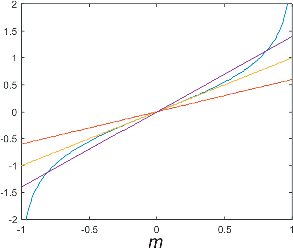
As shown in Fig. (9.2) for \(h = 0\) the straight lines with slopes larger 1 have three intersection points with the arctanh(\(m\)) curves (two symmetric with \(m \neq 0\)) while the straight lines with slopes smaller or equal
1 have only one intersection point at \(m = 0\). Since the slope is \(1/\tau\) obviously \(\tau = 1\) corresponds to the Curie temperature. For very large slopes, i.e. extremely small temperature, \(m = \pm 1\) are the intersection points and correspond to the saturation magnetization. For \(h \neq
0\) at least one intersection point will have \(m \neq 0\), which is the typical response of a para-magnet.
From a mathematical point of view either Eq. (9.4) or Eq. (9.5) can
be solved to find \(m(\tau)\). Solving the problem numerically only Eq. (9.4) is suitable, because brackening is a robust procedure for this type of function. Try Eq. (9.5); you will fail! This is a typical example
that one needs a basic understanding of strategies to solve problems numerically in order to translate the mathematical
problem into an efficient numerical algorithm. The following function is the working horse for our next jobs; it completely
follows the scheme of the function myzerosolv.
  function m = mymagnetization(tau, h, mstart)
     m = tau;
     for i=1:length(tau)
     myzerovar = tau(i);
     m(i) = fzero(@myzerofun, mstart);
     mstart = m(i);
     end

     function y = myzerofun(x)
       y=x-tanh((x+h)./myzerovar);
     end

  end
Let us summarize: For \(\tau = 0\) (and \(h = 0\)) we know the
analytical solutions \(m = \pm 1\) and \(m = 0\). This are the three branches we will again draw,
of course by starting close to \(\tau = 0\) because we will update the starting point for zero-finding as before.
We can not chose \(tau = 0\) in the numerical calculation because this will lead to an overflow error.
Your next job: Create a function which draws the three magnetization branches vs. \(\tau\) for \(h
= 0\). Include a line at \(m = 1/3\) into the graph. To calculate the temperature \(\tau\) of
the intersection point between the magnetization curve and the \(m = 1/3\) line will be the real job. For this
we will use cubic spline interpolation (see section 2.5). Check MATLAB-HELP for the appropriate example; copy the corresponding lines and create a function
like the following
  function my_cubic_spline_test
     x = -4:1:4;
     y = [0 .15 1.12 2.36 2.36 1.46 .49 .06 0];
     cs = spline(x,y);
     xx = -4:0.05:4;
     yy = ppval(cs,xx);
     plot(x,y,’o’,xx,yy,’-’);
  end
Your next jobs:
Call my_cubic_spline_test and play around to learn the details of this function
Create a function which draws the magnetization branches starting with \(m = 1\) vs. \(\tau\) for \(h = 0\), 0.1 and 1.0. Add the line \(m = 1/3\)
Incorporate the relevant parts of the above cubic spline example to interpolate the three curves.
Add the nested function
  function y = m_1_3(x)
          y = ppval(cs,x)-1./3;


      end
Use a call of fzero to calculate the temperatures \(\tau_{1/3}\) of the intersection points, i.e. \(m(\tau_{1/3}) = 1/3\)
Create a function which calculates \(\tau_{1/3}\) for an input array of \(h\) values and plot the curve; you will find a straight line!
Explain, why a simple straight line is found and discuss a more simple strategy to so calculate \(\tau_{1/3}\) vs. h.
HOMEWORK 4
Complete the jobs if you
did not finish in the lecture.
You must be able to discuss the details of your function!
© J. Carstensen (Comp. Math.)