9.2 Exercise 2

In this exercise we deal with numerical zero finding. Zero finding is one of the most important numerical procedures since e.g. solving equations is translated into a zero-finding problem. The theoretical concepts are discussed in section 3.1 through 3.5.
We start with the example

This equation cannot be solved analytically for arbitrary values of \(a\). Of course for \(a=0\) the solutions are well known: \(x_0 = (n + 1/2) \pi\). We will take much benefit of this analytical solutions (as nearly always when solving numerical problems!). Graphically one solves such equations by drawing the cos-function and the straight line with slope \(a\) in one graph. The intersection points between both curves are the solutions of our problem. Do it and learn more about the mathematical nature of our problem. You will need it!
For solving the problem numerically we first have to translate this equation into a zero-finding problem. The zeros of

are the solutions of our above equation.
As starting point we use the MATLAB function below:

 function y = myzerosolv(x)
    y = x;
    for i=1:length(x)
      myzerovar = x(i);
      y(i) = fzero(@myzerofun, pi.*0.5);
    end

   function y = myzerofun(x)
     y=cos(x)-myzerovar.*x;
   end

 end

Just download it. As typically the variable-name of the input array is \(x\) and the output-name is \(y\). The program calculates the zeros of the function \(f\) for an array of slope values \(a\). Details will be discussed soon. First we will execute the function:
So you have to predefine an array of slope values in the command window, e.g. a = 0:0.1:10. You can call the function from the command window as x0 = myzerosolv(a); and plot the result using plot(a, x0).
The most decisive part in the function myzerosolv is the call of the MATLAB function fzero. Check the MATLAB-help for the meaning of the two input parameter! Generate now the solutions for the second branch, i.e. solutions around pi.*1.5. You will recognize that for larger values of \(a\) the solutions are just those as for the branch starting at pi.*0.5. Additionally you will recognize that the solutions are not stable, i.e. there seem to be strongly different solution for neighboring \(a\)-values. But this is just an artifact of (nearly all) numerical zero-finding procedures. The ”brackening” as the first step in zero-finding does not work properly when the starting point for zero finding is far of the solution. We can drastically improve our algorithm by updating the starting point after each loop, since our \(a\)-values in the array increase continually with small changes. Simultaneously we can take the start-value as a second input parameter in our function to be more flexible:

 function y = myzerosolv(x, x0_start)
    y = x;
    for i=1:length(x)
      myzerovar = x(i);
      y(i) = fzero(@myzerofun, x0_start);
      x0_start = y(i);
    end

   function y = myzerofun(x)
     y=cos(x)-myzerovar.*x;
   end

 end

Before going on we will now discuss all details in the above function. The meaning of input and output parameter should be known by now! The command y = x; is preallocating the variable y, which is very important for execution speed. MATLAB will give a warning when this line is forgotten. for i=1:length(x) ... end is the syntax of a ”for”-loop in MATLAB. i is the loop variable starting with 1 and ending with length(x) which indicates the last element of x. All commands until end will be executed in each loop run. So the variable myzerovar takes successively all values of the array x and is constant for each call of the zero-finding procedure fzero. @myzerofun is the standard version of MATLAB to reference on functions as variables. Here myzerofun is a nested function, i.e. it is defined following the call of the function. This should be the standard in MATLAB and preferred to nested variables which would be the second approach to solve our problem: Either the variable myzerovar is not known when defining the function myzerofun or vice versa. x0_start = y(i) is updating the start parameter for fzero in the next iteration by the solution of the last iteration. The command line function y = myzerofun(x) needs more discussion; here the variables x and y are defined once more. The concept of ”shadowing” is used to define which variable x is meant: within the second function ... end block the second definition of x is used; it is ”shadowing” the outer definition of x.
Your next jobs:

• Create a new function which draws the three branches at pi.*0.5, pi.*1.5, and pi.*2.5. Do not (!) copy any part of myzerosolv into this new function; only call myzerosolv several times.

• Add in your function the branches for negative slopes. This will only work easily if you double check all relevant parts of the programming once more; it needs a small trick to work!

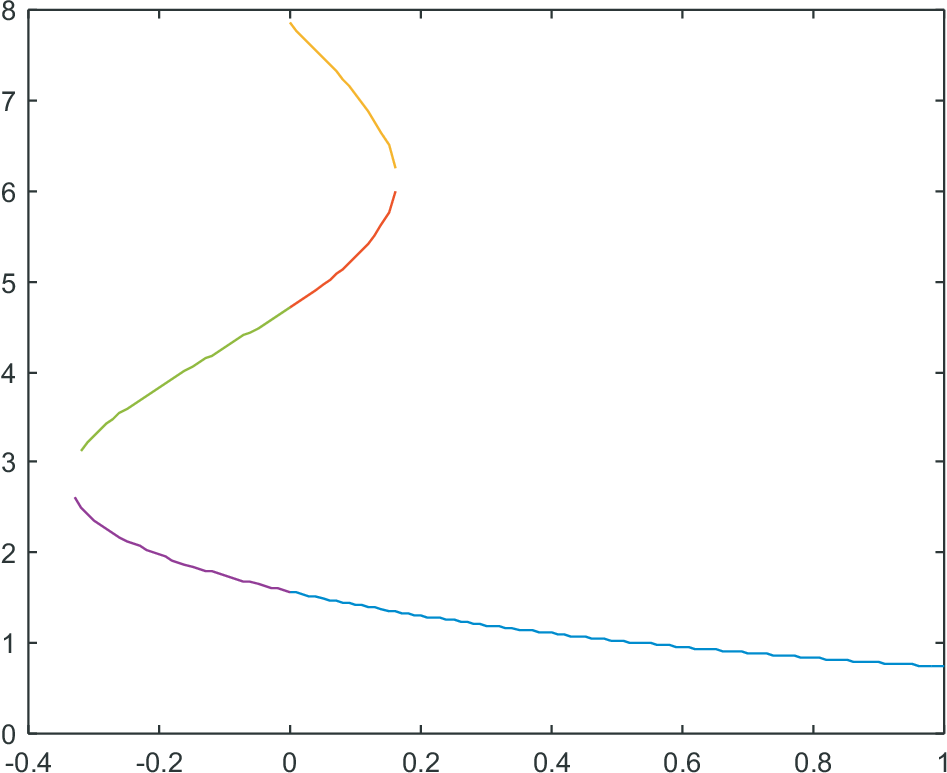
• You will recognize that your graph shows parts as solutions which belong to different branches. Write a ”cut”-function which removes the wrong parts of the calculated graphs, i.e. with function [ yn, an ] = cut( y, a ) ... end. So do not change the original function myzerosolv to solve the problem, but manipulate just the resulting data (y, a) into ’cut data’ [yn, an].

Your final result should look somehow like shown in Fig. 9.1.

HOMEWORK 3
Write a zero finding function

1. With input \(a\) and output the numerical zero value and the approximate solution (see below).

2. For the equation \(\sin(x) = a \,x^2\).

3. Use the linear approximation of the sin-function to find the approximate solution \(x = 1 / a\).

4. Compare the numerical solution with the approximate solution for different values of \(a\).

You must be able to discuss the details of your function!

© J. Carstensen (Comp. Math.)