Ferromagnetism in ”mean-field” approximation

5.4 Ferromagnetism in ”mean-field” approximation

As an important result of chapter 4 we found that magnetic ordering (without external fields) only occurs if electrons are strongly coupled.
A description of a state within the Fermi statistics according to Eq. (5.7) is only possible if electrons are not coupled strongly.
In the following we will handle the magnetic moment of a single electron and its interaction with other electrons like an external magnetic field. We substitute the coupling between electrons by a mean magnetic field of all electrons which act on one electron. This allows to assume the electrons to be independent; we just have to calculate the magnitude of the mean induced magnetic field.
The additional energy of an electron with spin parallel or antiparallel in an external magnetic field is defined by:

\begin{equation*} E = - \vec{M}_L \vec{B} = \frac{g_s e}{2 m_e} \vec{S} \vec{B} = \pm \frac{1}{2} \hbar \frac{g_s e}{2 m_e} \mu_0 |H_{eff}| \label{e_mag} \end{equation*}

(5.8)

with

\begin{equation*} H_{eff} = H + M \end{equation*}

(5.9)

\(H\) is an external magnetic moment; \(M\) is the self induced moment of all electrons.
The electron in the state \(j\) with spin up has the energy

\begin{equation*} E_{\uparrow}= E_{j,0} + \mu_H (H + M) \end{equation*}

(5.10)

The electron with spin down has an energy

\begin{equation*} E_{\downarrow}= E_{j,0} - \mu_H (H + M) \end{equation*}

(5.11)

For the following we will assume that each lattice point is occupied with exactly one electron with spin up or spin down. This occurs often in solids since the strong coulomb repulsion hinders electrons to move freely in the solid.
The occupation probability is

\begin{equation*} W_{j\uparrow} \propto \exp \left(- \frac{E_{j,0}- \mu + \mu_H (H + M)}{kT} \right) \end{equation*}

(5.12)

and

\begin{equation*} W_{j\downarrow} \propto \exp \left(- \frac{E_{j,0}- \mu - \mu_H (H + M)}{kT} \right) \qquad . \end{equation*}

(5.13)

\begin{equation*} W_{j\uparrow} = \frac{ \exp \left(- \frac{E_{j,0}- \mu + \mu_H (H + M)}{kT} \right) } {\exp \left(- \frac{E_{j,0}- \mu + \mu_H (H + M)}{kT} \right) +\exp \left(- \frac{E_{j,0}- \mu - \mu_H (H + M)}{kT} \right) } \label{w_up} \end{equation*}

(5.14)

and

\begin{equation*} W_{j\downarrow} = \frac{ \exp \left(- \frac{E_{j,0}- \mu - \mu_H (H + M)}{kT} \right) } {\exp \left(- \frac{E_{j,0}- \mu + \mu_H (H + M)}{kT} \right) +\exp \left(- \frac{E_{j,0}- \mu - \mu_H (H + M)}{kT} \right) } \label{w_down} \end{equation*}

(5.15)

From the equations (5.14) and (5.15) we calculate the expectation value for a magnetic moment:

\begin{equation*} M = M_0 \left( W_{j\uparrow} - W_{j\downarrow} \right) = \frac{ \exp \left(- \frac{E_{j,0}- \mu + \mu_H (H + M)}{kT} \right) - \exp \left(- \frac{E_{j,0}- \mu - \mu_H (H + M)}{kT} \right)} {\exp \left(- \frac{E_{j,0}- \mu + \mu_H (H + M)}{kT} \right) +\exp \left(- \frac{E_{j,0}- \mu - \mu_H (H + M)}{kT} \right) } \qquad , \end{equation*}

(5.16)

i.e.

\begin{equation*} M = \frac{ \exp \left(- \frac{+ \mu_H (H + M)}{kT} \right) - \exp \left(- \frac{- \mu_H (H + M)}{kT} \right)} {\exp \left(- \frac{+ \mu_H (H + M)}{kT} \right) +\exp \left(- \frac{- \mu_H (H + M)}{kT} \right) } \label{rel_mag} \end{equation*}

(5.17)

where \(M_0\) is the magnetization in case of saturation.
For calculating \(M\) self consistently we get the following equation

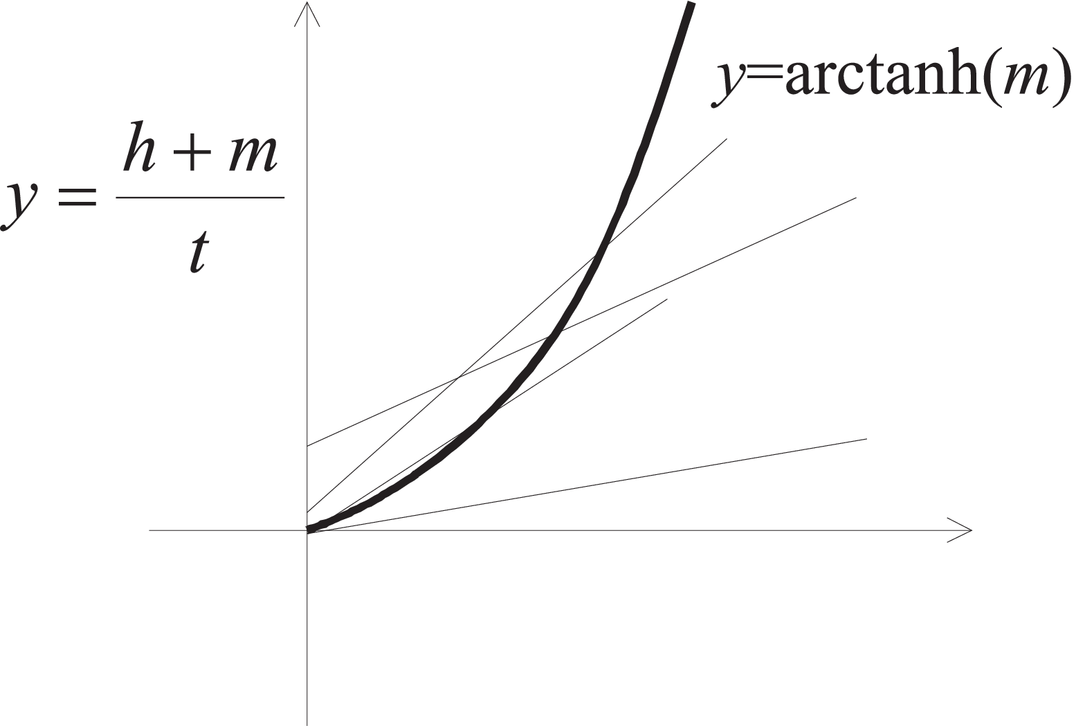
\begin{equation*} m = \tanh \left( \frac{h+m}{t} \right) \qquad , \end{equation*}

(5.18)

respectively

\begin{equation*} \mbox{arctanh}(m) = \frac{h+m}{t} \qquad . \end{equation*}

(5.19)

The graphical solution of Eq. (5.18) shows that applying an external magnetic field \((h\gt 0)\) we always find a crossing of both graphs, i.e. a magnetization exists (paramagnetism). Spontaneous magnetization \(H=h=0\) (ferromagnetic ordering) we only find, if \(1/t\gt 1\) holds, i.e. at low temperatures.