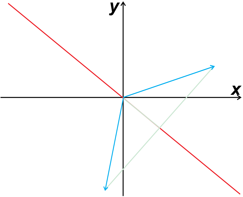
mirroring on the (1, -1)-plane

mirroring on the (1, -1)-plane
Before discussing the general mathematical procedure to calculate Eigenvalues and Eigenvectors we will discuss a very illustrative example which highlights that the concept of Eigenvectors is not just a mathematical game but a general concept which everybody uses (implicitly) for describing e.g. geometrical transformation. The above figure shows the the transformation of a vector by mirroring on the (1, -1)-plane. This transformation can only be understood and described by discussing two projections of the vector: (i) on the plane, and (ii) perpendicular to the plane. While the first projection does not change, the second projection translates into it’s negative when mirroring. So obviously mirroring is a linear operation and we found two vectors, which just change there length (not there orientation) when applying the mirror transformation, i.e. we found two Eigenvectors and they are essential to discuss the action of a mirror. For the example above we found without any calculation the Eigenvectors and Eigenvalues
| \[\begin{array}{cc} \mbox{Eigenvector} \quad \left(\begin{array}{c}+1\\-1\end{array}\right)& \mbox{ for Eigenvalue} \quad \lambda = +1\\ & \\ \mbox{Eigenvector} \quad \left(\begin{array}{c}+1\\+1\end{array}\right)& \mbox{ for Eigenvalue} \quad \lambda = -1\\ \end{array}\] |
To apply the general mathematical treatment for finding Eigenvalues and Eigenvectors we first have to find the matrix representing the mirroring on the (1, -1)-plane. Since we are dealing with a linear transformation it is enough the check for the transformation of the two base vectors. We directly find:
| \[\begin{array}{cc} \mbox{base vector 1} \quad \left(\begin{array}{c}1\\ 0\end{array}\right)& \mbox{ transforms into} \quad \left(\begin{array}{c}0\\-1\end{array}\right)\\ & \\ \mbox{base vector 2} \quad \left(\begin{array}{c}0\\ 1\end{array}\right)& \mbox{ transforms into} \quad \left(\begin{array}{c}-1\\ 0\end{array}\right)\\ \end{array}\] |
so we get
| \[\begin{array}{ccc} \tilde M & = & \left(\begin{array}{cc}0&-1\\-1&0\end{array}\right) \end{array}\] |
Solving for
| \[\det(\tilde M-\lambda\tilde I)=0\] |
we get the characteristic polynom
| \[0 = \lambda^2-1\] |
with the (as already from the above discussion expected) solutions
| \[\lambda_{1,2}= \pm 1\] |
For \(\lambda_1 = 1\) we find
| \[ \left(\begin{array}{cc}-1&-1\\-1&-1\end{array}\right)\left(\begin{array}{c}v_1\\ v_2\end{array}\right)=\left(\begin{array}{c}0\\ 0\end{array}\right)\quad\mbox{i.e.}\quad \vec{v}_1=v_1\;\left(\begin{array}{c}1\\-1\end{array}\right).\] |
For \(\lambda_1 = -1\) we find
| \[ \left(\begin{array}{cc}1&-1\\-1&1\end{array}\right)\left(\begin{array}{c}v_1\\ v_2\end{array}\right)=\left(\begin{array}{c}0\\ 0\end{array}\right)\quad\mbox{i.e.}\quad \vec{v}_2=v_2\;\left(\begin{array}{c}1\\1\end{array}\right).\] |
In order to get an orthonormal set of base vectors we can take
| \[\begin{array}{ccc} \vec{v}_1=\left(\begin{array}{c}\frac{1}{\sqrt{2}}\\-\frac{1}{\sqrt{2}}\end{array}\right) & \quad \mbox{and} \quad & \vec{v}_2=\left(\begin{array}{c}\frac{1}{\sqrt{2}}\\ \frac{1}{\sqrt{2}}\end{array}\right)\end{array} \] |
Putting \(\vec{v}_1\) and \(\vec{v}_2\) as column vectors into a matrix \(\tilde{U}\) we get a unitary matrix
| \[ \tilde{U} = \left(\begin{array}{cc}\frac{1}{\sqrt{2}}&\frac{1}{\sqrt{2}}\\-\frac{1}{\sqrt{2}}&\frac{1}{\sqrt{2}}\end{array}\right)=\left(\begin{array}{cc}\vec{v}_1&\vec{v}_2\end{array}\right) \] |
Obviously
| \[ \tilde{U}^+ = \left(\begin{array}{cc}\frac{1}{\sqrt{2}}&-\frac{1}{\sqrt{2}}\\ \frac{1}{\sqrt{2}}&\frac{1}{\sqrt{2}}\end{array}\right)=\left(\begin{array}{c}\vec{v}_1^+\\\vec{v}_2^+\end{array}\right) \] |
so \(\tilde{U}^+\tilde{U}=\tilde{I}\) since \(\left\langle v_i\right|v_j\rangle =\delta_{ij}\) (i.e. \(\tilde{U}^+ = \tilde{U}^{-1}\)) and
| \[ \tilde{U}^+\tilde{M}\tilde{U}=\left(\begin{array}{cc}1&0\\ 0&-1\end{array}\right)=\left(\begin{array}{cc}\lambda_1&0\\ 0&\lambda_2\end{array}\right)\] |
The statements related to \(\tilde{U}\) are just examples for the general results for Hermite matrices as discussed later in section 2.16.
© J. Carstensen (Math for MS)