As follows from the above remarks, it suffices to consider a first-order ODE for a single-valued function,
|
| \begin{equation*} \label{eq:ODE1} \frac{{\rm d}y}{{\rm d}x} = f(x,y), \end{equation*} | (7.5) |
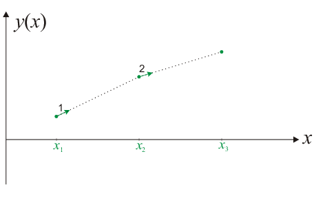
in order to be able to solve all ODE problems. The simplest way to solve such an equation is to use the local slope, which is given by the right-hand side of Eq. (7.5) and which is always known in an initial-value problem, to linearly extrapolate the function and estimate the function value a certain step size away from the starting point. With the new function value at hand, a new slope can be calculated. So the procedure can be repeatedly applied.
Therefore, to proceed from the \(n\)-th position on the \(x\) axis, \(x_n\), to the next position \(x_{n+1} = x_n + h\), one simply has to increment the function value by “step size times slope” (cf. Fig. 7.1):
|
| \begin{equation*} y_{n+1}=y_n+hf(x_n,y_n). \end{equation*} | (7.6) |
Obviously, for this method the step size must be rather small in order to avoid numerical errors.

© J. Carstensen (Comp. Math.)