Linear Least Squares: Example and remark

4.5 Linear Least Squares: Example and remark

Example: straight line
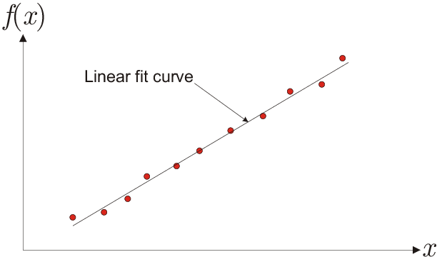
The model function for a straight line is \(f(x)=ax+b\), which depends linearly on the two parameters \(a\) and \(b\). Consider the eleven given data points shown in Fig. 4.3(a) that are to be fitted by a straight line. Here, the “model vector” can be written as

\begin{equation*} {\left(\begin{array}{c} m_1 \\ m_2 \\ \vdots \\ m_{11} \end{array}\right)} = {\left(\begin{array}{cc} x_1&1 \\ x_2&1 \\ \vdots & \vdots \\ x_{11}&1 \end{array}\right)} ^{\vec{M}} {\left(\begin{array}{c} a \\ b \end{array}\right)}, \end{equation*}

(4.22)

i.e., M is an \(11\times2\) matrix with a column of constant values of 1 corresponding to parameter \(b\).

(a) (b)

Figure 4.3: (a) Fitting a straight line to given data points. (b) Comparison of fitting results for the usual least squares minimization (“square function”) and robust fitting using the absolute value of the differences (“abs function”).

Remark: robust fitting
Obviously, since they minimize that function, the fitting parameter values obtained depend on the objective function used, which will influence the fitting result. This is of importance in the following situation: When fitting experimental data it may happen that a few data points lie noticeably far away from the expected model curve, which will lead to a large contribution of these points in the \(\chi^2\) function. As a consequence, the fitted curve will be drawn close to these points in order to minimize the gap. However, from the point of view of an experimentalist, it is not desirable that a few points that can be considered an exception have a large influence on the result.

To reduce the influence of data points with large deviations from the model curve, a linear objective function can be used instead of the \(\chi^2\), which is called robust fitting:

\begin{equation*} \label{eq:chi_abs} \chi_{\text{abs}}(\vec{a})= \sum^n_{i=1}{\left|y_i-f(x_{i},\vec{a})\right|}. \end{equation*}

(4.23)

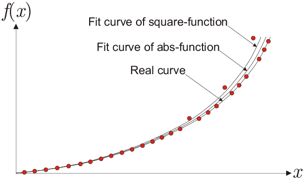
The main difference between \(\chi_{\text{abs}}\) and \(\chi^2\) (Eq. 4.15) is that \(\chi^2\) can be differentiated at all values while \(\chi_{\text{abs}}\) does not have derivative everywhere. To illustrate the influence of using \(\chi_{\text{abs}}\) instead of \(\chi^2\), Fig. 4.3(b) shows a constructed example of fitting a parabola where a few data points are shifted upwards. Obviously, the \(\chi^2\) result deviates stronger from the true parabola.